3 줄 요약
- Offline : 성능을 위해 최대한 욱여넣음
- Complex domain spectral mapping
- DNN + Beamforming + DNN + Beamfroming
ABSTRACT
제안 :
single- & multi-channel complex spectral mapping
direct-path 신호의 real & image 성분을 각각 추정
두개의 DNN
- single-channel complex spectral mapping : 출력을 MVDR Beamformer에 사용
- 빔포밍 결과의 RI 성분은 공간정보를 담고 있기 때문에 mixture의 RI 성분과 결합하여 두번째 mutil-channel spectral mapping에 사용한다.
추정된 spectrum으로 time-varying beamforming 또한 사용하였다.
1. INTRODUCTION
- Problem
- 잡음과 반향같은 interference 들이 ASR(Automatic Speech Recognition) 성능을 저하시킨다.
- History보통은 다중 채널 빔포밍 이후에 후처리 필터를 사용하는데, Wiener filter + MVDR, real value post filter를 사용한다. 이런 방식은 타겟 방향, 음성과 잡음의 PSD(Power Spectral Density), 공분산 행렬이 필요하다. 주로 GCC-PHAT[5] 같은 Localization, 전통적인 음성 향상 기법[3], Spatial Clustering 같은 BSS(Blind Source Separation)[6][7] 을 통해 구한다.
- 최근엔 DNN기반의 TF masking 또는 mapping이 enhancement와 separation의 주류가 되었다. Mask (or magnitude) 추정은 DNN을 통해 굉장한 향상을 보였다. 최근의 CHiME-4 challenge 의 상위 팀들은 TF masking 과 딥러닝 기반의 빔포밍을 사용하였다.[10]
- speech enhancement와 source separation에서 공간 정보를 활용하기 위해 다중 마이크를 사용한다.
- Background of this paper기존의 TF masking 기반의 빔포밍은 주로 spatial covariance를 masking을 한 mixture의 summation 으로 구했다. [6],[9].[11]-[14]이러한 상황에서 - 믿기로는 - magnitude estimation에 더불어 phase estimation과 covariance matrix를 위한 추정된 complex spectra 를 사용하는 것이 도움이 될 것이다. (두번째 모델)빔포밍이 일반적으로 phase를 향상시키지만 마이크의 수에 의존하고 강한 반향에 약하다. 후처리 필터를 위해서 phase estimation을 해서 빔포밍된 phase를 향상 시킬 수 있다. 현대의 ASR들은 magnitude-based features 만 사용하지만 정확한 phase estimation은 ASR 성능 향상에 간접적인 도움을 준다.
- Contributions
- complex spectral mapping 을 위한 magnitude-domain loss를 제안한다. PESQ를 향상 시킨다.
- complex spectra 가 magnitude-domain mask estimation 보다 beamforming에 통계적으로 더 좋다.
- time-varying beamforming을 위한 estimated complex spectra을 사용하는 새로운 방법을 제안한다.
- CHiME-4 에 대한 SOTA의 enhancement와 ASR을 제공한다.
- 본 연구는 complex domain 에서[18] complex spectral mapping[19],[20] 을 통해서 단일 채널 무반향상황 가정 이었던 이전 작업을 넘어 새로운 loss function 과 multi-channel 을 사용한다.
- 이 방법은 단순히 weighting mechanism을 사용하는 것이 아니다. 일반적으로 후처리 필터는 magnitude 만 사용하는데, 이러면 phase inconsistency를 피할 수 없고[15]-[17], time domain에 correspond하지 않게 된다.
- 하지만 잡음과 반향이 강한 상황에서 TF bin에 target speech가 dominant 하지 않을 수 있다. TF bin 에는 필연적으로 잡음과 반향이 들어 있을 수 밖에 없다.
- magnitude mask 에서 더 나아가 phase estimation의 효과를 연구 하였다.
2. PHYSICAL MODEL AND OBJECTIVES
$P$ 개의 마이크의 신호를 STFT domain으로 변환하여 다음과 같이 표시할 수 있다.
$$\mathbf{Y}(t,f) = \mathbf{c}(f:q)S_q(t,f) + \mathbf{H}(t,f) + \mathbf{N}(t,f)\\=\mathbf{S}(t,f) + \mathbf{V}(t,f) \tag{1}$$
$S_q$ : direct-path signal
$\mathbf{c}$ : relative transfer function with the $q$th element being $1$
$\mathbf{H}$ : reverberation of direct-path signal
$\mathbf{N}$ : reverberant noise
$\mathbf{S}(t,f) :$ target speech
$\mathbf{V}(t,f) :$ non-target signal
화자는 움직이지 않는다고 가정한다.
offline processing 시나리오
sample variance를 normalize하고 시작함→ 신호의 random gain을 해결해주기 때문에 mapping 기반의 기법에는 중요하다.
제안된 알고리즘은 한번 학습되면 다른 종류의 배열에도 동작한다.
$\because$ Shared parameters 로 각 마이크별로 동작한다.
3. PROPOSED ALGORITHMS

- 1-ch noisy input ⇒ single channel spectral mapping
- every output of (1) ⇒ TI-MVDR
- 1-ch noisy input + 1-ch output of (2) ⇒ multi-channel complex spectral mapping
- every output of (3) ⇒ TI/TV-MVDR
- Note첫번째 MVDR 시 TV-MVDR 수행시 'not clearly better' 하다고 함 ⇒ 성능차이가 유의미하지 않다?
- (4) 를 제외하고는 모두 채널별로 각각 연산을 수행함
각 마이크 별로 direct-path signal의 phase가 다르기 때문에 빔포밍을 각각 수행한다.
A. Single-Channel complex Spectral Mapping
[18]-[20] 에 이어서 direct path signal의 RI 성분을 직접적으로 예측하기 위해서 다음과 같은 loss function을 사용한다.
$$\mathcal{L}_{RI} = || \hat{R}_P - \Re(S_P)||_1 + ||\hat{I}_P - \Im(S_P)||_1 \tag{2}$$
$p \in \{1, . . . , P\}$
$\hat{R}_p,\hat{I}_p$ : 예측한 RI 성분
$\hat{S}^{k}_p = \hat{R}^{k}_p + j\hat{I}^{k}_p$
$k \in \{1,2\}$ : DNN 모델
최근의 연구 [19],[27] 이 magnitude loss를 complex spectra approximation에 포함하였다.
$$\mathcal{L}{RI+Mag} = \mathcal{L}{RI} + \Large{||} \small \sqrt{\hat{R}^2_p + \hat{I}^2_p} -|S_p| \Large{||}\small_1 \tag{3}$$
Motivation은 magnitude estimation에 phase에서 만드는 에러만큼 $\mathcal{L}_{RI}$ 만으로눈 충분히 magnitude estimation을 할 수 없기 때문에 보완해줘야 한다는 것이다. [19],[27] 과 다른 것은 power 또는 Logarithmic compression을 하지 않는 것이다.
- Note
- 실험결과 $\mathcal{L}{RI}$ 보다 $\mathcal{L}{RI+Mag}$ 일 때 성능이 더 좋다,
B. Multi-Channel Complex Spectral Mapping
[6],[9],[11]-[14] 같이 TF mask로 weight 를 주는 것 보다는 직접적으로 추정된 complex spectral을 사용하여 covariance matrix 계산을 한다.
$$\hat{\mathbf{\Phi}}^{(s)}(f) = \frac{1}{T}\sum^T_{t=1}\hat{\mathbf{S}}(t,f)\hat{\mathbf{S}}(t,f)^H \tag{4}$$
$$\hat{\mathbf{\Phi}}^{(v)}(f) = \frac{1}{T}\sum^T_{t=1}\hat{\mathbf{V}}(t,f)\hat{\mathbf{V}}(t,f)^H \tag{5}$$
$\mathbf{\hat{V}} = \mathbf{{Y}} -\mathbf{\hat{S}}$ ㅣ
$T :$ the total number of frames
relative transfer function 은 다음과 같이 계산된다.
$$\hat{\mathbf{r}}(f) = \mathcal{P}\{\hat{\Phi}^{(s)}(f)\}\\\hat{\mathbf{c}}(f;q) = \hat{\mathbf{r}}(f)/\hat{r}_q(f) \tag{6}$$
$\mathcal{P}$ : the principal eigenvector
$\hat{r}_q(f)$ : $q$th element of $\mathbf{\hat{r}}(f)$
speech covariance matrix는 제대로 추정되었다면 rank-one matrix 이다. 따라서 principal eigenvector 를 steering vector 추정하는 것은 [11],[13],[3] 은 합리적인 추정이다.
$\hat{\mathbf{r}}(f)$ 를 각 마이크별로 $\hat{r}_q$ 로 나눠주는데, MVDR 수행 시 각 frequency 별로 random complex gain이 발생하는 것을 막아서 speech distortion 을 방지한다.
time-Invariance MVDR(TI-MVDR) 는 다음과 같이 구할 수 있다.
$$\hat{\mathbf{\omega}}(f;q) = \frac{ \hat{\mathbf{\Phi}}^{(v)}(f)^{-1} \hat{\mathbf{c}}(f;q) }{ \hat{\mathbf{c}}(f;q)^H \hat{\mathbf{\Phi}}^{(v)}(f)^{-1} \hat{\mathbf{c}}(f;q) } \tag{7}$$
- Note : MVDR (Minimum Variance Distortionless Response)
$$\mathbf{w}(f) =\argmin_{\mathbf{w}(f)}E\{|\mathbf{w}^H(f)\mathbf{u}(t,f)|^2\} \ \cdots \mathsf{Minimum \ Variance}\\\mathsf{subject\ to}\ \mathbf{w}^H(f)\mathbf{h}(f)=1 \cdots \mathsf{Distortionless}$$
$$\therefore \mathbf{w}(f) = \frac{\mathbf{R_u}^{-1}(f)\mathbf{h}(f)}{\mathbf{h}^H(f)\mathbf{R_u}^{-1}(f)\mathbf{h}(f)}$$
빔포밍을 통해
$$\widehat{BF}_q(t,f) = \mathbf{\hat{\omega}}(f;q)^H\mathbf{Y}(t,f)$$
을 얻는다.
두 번째 DNN 은 $\widehat{BF}_q(t,f)$ 의 RI 성분과 $Y_q$ 를 사용하여 $S_q$를 추정한다.
$\widehat{BF}_q(t,f)$ 는 spatial feature[28]-[32] 로 볼 수 있다. 이는 complex domain에서 수행되기 때문에 기존의 real domain에서 수행된 기법
(IPD(inter-channel phase differences)s[33], cosine and sine IPDs[29][34], target direction compensated IPDs[25], magnitudes of beamformed mixtures[32])
보다 phase estimation에서 좋은 성능을 보인다.
MVDR이 distortion을 거의 일으키지 않기 때문에 두번째 DNN이 direct-path signal을 예측하는데 도움을 줄 수 있다. 다른 beamformer들, MCWF(Multi-channel Wiener filter) 나 GEV(Generalized Eigenvector Beamforming) 은 같은 projection direction(i.e. $\hat{\mathbf{\Phi}}^{(v)}(f)^{-1} \hat{\mathbf{c}}(f;q)$ ) 을 사용하지만, 다른 spectral gain을 noise suppression에 사용한다. 이러한 gain은 speech distortion을 일으킨다. 따라서 우리는 왜곡이 없는 MVDR을 사용한다.
C. Adaptive Covariance Matrix Computation
화자가 고정되었다고 가정하기 때문에 전체 프레임에서 추정하는 것이 합리적이다. 하지만 화자가 고정되어 있더라도 환경은 실제 상황에서 굉장히 time-varying 하기 때문에 - BUS, CAF in CHiME4 - 따라서 Noise Covariance matrix 를 TF unit 마다 또는 block 마다 하는 것이 필요하다.
[35] Y. Kubo, T. Nakatani, M. Delcroix, K. Kinoshita, and S. Araki, “Maskbased MVDR beamformer for noisy multisource environments: Introduction of time-varying spatial covariance model,”
최근에 [35] 제안된 알고리즘을 따라서 Time-varying noise covariance matrices를 추정한다.
per-frequency T-F mask based covariance matrix를 maximum a posterior framework에서 a prior로 본다.
prior 와 masking된 mixture의 weighted combination으로 공분산을 구한다.
$$\hat{\mathbf{\Phi}}^{(v)}(t,f)\\ = (1-\alpha) \frac{\sum^{t+\Delta}{t-\Delta} \hat{\mathbf{V}}(t,f)\hat{\mathbf{V}}(t,f)^H }{trace( \sum^{t+\Delta}{t-\Delta} \hat{\mathbf{V}}(t,f)\hat{\mathbf{V}}(t,f)^H ) / P} \\+ \alpha\frac{\hat{\mathbf{\Phi}}^{(v)}(f)}{ trace (\hat{\mathbf{\Phi}}^{(v)}(f))/P} \tag{8}$$
$\alpha :$ 실험적으로 0.5 로 설정
$\Delta$ : window의 반으로 설정
$\Delta$ is half the window size in frames.
Q : $\Delta$ 의 크기는 window가 512이면 256인가?
⇒ [35] 에는 block 단위로 구성하였다. 아마 $\Delta$는 한 프레임이지 않을까
뒤에서도 frame 단위로 설명하고 있다.
[35] 는 mask를 사용하지만 본 논문은 complex spectral mapping 을 사용하는 차이가 있다.
이를 통해 더 정확한 공분산 추정을 할 수있다. 추가로 time-varying PSD의 효과를 상쇄하기 위해서 계산 전에 energy level을 normalize 한다. noise PSD가 굉장히 non-stationary 하기 때문에 두 항 중 하나가 dominant할 수가 있기 때문이다.
첫번째 항이 $2\Delta+1$ 프레임 만큼의 작은 context를 다루고 두번째 항이 전체 프레임을 다룬다. 이를 통해 long-term stationary 정보를 사용하면서도 갑작스런 잡음 특성의 변화에 적응 할 수 있게 된다.
Time-varying MVDR (TV-MVDR) 은 다음과 같이 구할 수 있다.
$$\hat{\mathbf{\omega}}(t,f;q) = \frac{ \hat{\mathbf{\Phi}}^{(v)}(t,f)^{-1} \hat{\mathbf{c}}(f;q) }{ \hat{\mathbf{c}}(f;q)^H \hat{\mathbf{\Phi}}^{(v)}(t,f)^{-1} \hat{\mathbf{c}}(f;q) } \tag{9}$$
실험에서 $\Delta$ 를 2-mic 일 떄는 0, 6-mic 일 때는 3으로 하였다.
$\Delta$ 가 0 일 때 잡음제거를 더 많이하고 들기 더 좋았다. 하지만 이런 잡음 추정이 항상 정확하지는 않았다. 6채널 상황에서 MVDR은 더 많은 자유도를 가지고 부정확한 잡음 추정의 enerygy를 낮춰서 왜곡을 유발 할 수 있다.
따라서 $\Delta$를 높혀서 더 안정적으로 공분산을 구해서 잡음 제거를 희생하여 왜곡울 줄였다. 2채널 상황에서 $\Delta$를 0으로 둬도 잡음 제거가 제한적이기 때문에 왜곡이 거의 생기지 않는다.
4. EXPERIMENTAL SETUP
CHiME-4 corpus[4] 를 대상으로 1,2,6 마이크 상황에서 ASR을 수행.
각각의 DNN 출력 $\hat{S}^{(1)}_q, \hat{S}^{(2)}_q$ 를 speech enhancement
각각의 Beamforming 출력 $\widehat{BF}^{(1)}_q,\widehat{BF}^{(2)}_q$ 을 speech recognition 을 위해 사용.
$\because$ 빔포밍은 DNN보다 잡음을 덜 제거하지만 왜곡이 적어서 ASR에 유리
A. CHiME-4 Corpus
Computational Hearing in Multi-source Environments.
(CHiME-4 설명)
- Real data에는 녹음 안된 채널이 있는 데이터가 있다고함
- 앞 쪽의 2-채널 에는 전체 데이터에 대해서 문제가 없어서 2-마이크 상황에선 그냥 사용
- 6-마이크 상황에서는
we first select a microphone signal that is most correlated with the other five, and then throw away the signals with less than 0.3 correlation coefficients with the selected signal.
Q : 6채널에서 어떻게 해결하는가?
가장 덜 상관있는 채널을 버린다? 그러면 6채널이 안되는데
B. Frontend Enhancement System

Q : 두번째 DNN은 어떻게 돌아가는가
⇒ Fig 2 와 같은 구조, 입력 채널만 다르다
⇒ 첫번째 DNN 은 1 채널, 2번째 DNN은 2채널(multi : 첫번쨰 MVDR 결과와 noisy inpu)
5번 마이크가 가장 SNR이 높게 나오기 때문에 reference 마이크로 설정하였다.
- Network
- TCN[36] ⇒ long term temporal dependency
- UNet[37] 과 유사 : skip connections, dens blocks[38],[39]
- linear activation in output layer
- Swish non-linearity(2017)
Swish Activation Function by Google
Searching for Activation Functions
$$f(x) = x \cdot \mathsf{sigmoid}(\beta x)$$

tends to work better than ReLU on deeper models across a number of challenging datasets
$\beta$ 값을 명시하지는 않음
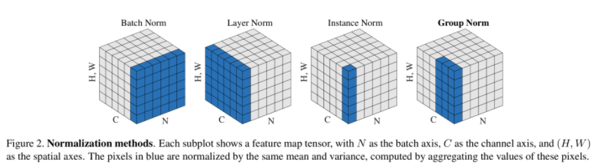
- Instance normalization(IN) (2017)
단일 데이터(instance)에 대해서 Normalization
Instance Normalization: The Missing Ingredient for Fast Stylization

This prevents instance-specific mean and covariance shift simplifying the learning process.
- Dilated Convolution
2D convolution using a 3 kernel with a dilation rate of 2 and no padding
모델 구성 요소를 왜 이렇게 정했는 지는 선행 논문 [13],[23]-[26]들을 봐야 알 수 있을 것 같다.
각 모델은 13M params
- setting
- frame length : 32 ms
- shift length : 8 ms
- sampling rate : 16kHz
- FFT size : 512
각 채널에 대해서 normalize 수행
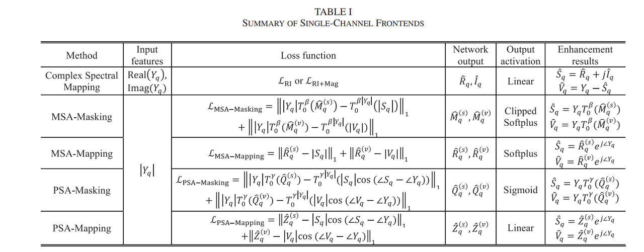
C. Baseline Frontend System
- MSA(Magnitude Spectrum Approximation)[1]
- PSA(Phase-sensitive Spectrum Approximation)[42]
Fig 2 와 같은 모델 사용. 입출력 feature와 activation 만 다름
TI-MVDR 을 위해선 다음과 같이 공분산을 구함
$$\hat{\Phi}^{(d)} (f) = \frac{1}{T} \sum^T_{t=1}\eta^{(d)}(t,f)\mathbf{Y}(t,f)\mathbf{Y}(t,f)^H \tag{10}$$
where
$d \in \{s,v \}$
PSA masking 에서는
$$\eta^{(d)} = \mathsf{median} (\frac{T^\beta_0(\hat{M}_1^{(d)})}{T^\beta_0(\hat{M}_1^{(s)}) + T^\beta_0(\hat{M}_1^{(v)}) } , ... \frac{T^\beta_0(\hat{M}_P^{(d)})}{T^\beta_0(\hat{M}_P^{(s)}) + T^\beta_0(\hat{M}_P^{(v)}) } ) \tag{11}$$
MSA masking 에서는
$$\eta^{(d)} = \mathsf{median} (T^\gamma_0(\hat{Q}_1^{(d)}) , ... , T^\gamma_0(\hat{Q}_P^{(d)}) ) \tag{12}$$
where
$\beta = 5.0$
$\gamma = 1.0$
CHiME-4 task 에서 microphone failure가 있기 때문에 median pooling 으로 해결 하였다.
Q : $T_0$ ?
⇒ 지수승을 하는 걸 보니까 scalar 같은데, 함수처럼 표현하고 있다. notation 자체는 시간일 텐데
따라서 complex spectral mapping 시에도(TI-MVDR시) 다음과 같이 공분산을 계산한다.
$$\hat{\Phi}^{(s)}(f) = \frac{1}{T} \sum^T_{t=1} \eta^{(s)}(t,f)\hat{\mathbf{S}}(t,f)\hat{\mathbf{S}}(t,f)^H \tag{13}$$
$$\hat{\Phi}^{(v)}(f) = \frac{1}{T} \sum^T_{t=1} \eta^{(v)}(t,f)\hat{\mathbf{V}}(t,f)\hat{\mathbf{V}}(t,f)^H \tag{14}$$
where
$$\eta^{(s)} = \mathsf{median}(\frac{|\hat{S_1}|}{|\hat{S_1}| + |\hat{V_1}|} , ...\frac{|\hat{S_P}|}{|\hat{S_P}| + |\hat{V_P}|} ) \tag{15}$$
$$\eta^{(v)} = \mathsf{median}(\frac{|\hat{V_1}|}{|\hat{S_1}| + |\hat{V_1}|} , ...\frac{|\hat{V_P}|}{|\hat{S_P}| + |\hat{V_P}|} ) \tag{16}$$
(10) 과 달린 (13),(14) 는 mixture가 아닌 추정된 speech와 noise에서 공분산을 계산한다.
2-마이크 상황에서는 마이크 실패가 없기 때문에 이 방법은 6-마이크 상황에서만 사용한다.
D. backend Recognition System
DNN-HMM 기반의 ASR 시스템
CHiME-4 training set 으로 학습
80d -log Mel feature 사용, delta, double delta
acoustic model : Wide-residual BLSTM
...
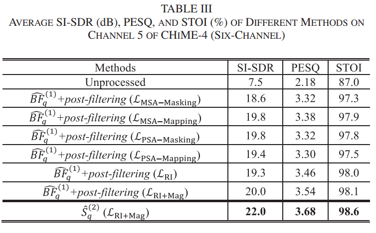
5. EVALUATION RESULTS
SI-SDR(scale invariant signal-to-distortion ratio)
PESQ(Perceptual Evaluation of Speech Quality)
STOI(short-time objective intelligibility)
A. Enhancement Performance
단계 진행시 이전 단계에서 가장 좋았던 설정을 이용
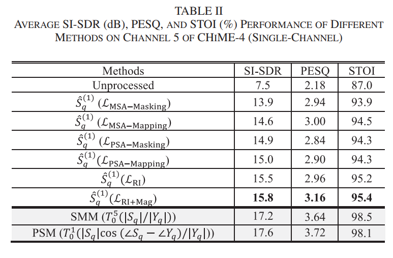
최하단의 2 항목은 'oracle magnitude domain' ⇒ Ideal 에서 수행한 것

[46] - 2018 IWAENC : BLSTM + MVDR
[47] - 2018 APSIPA ASC : CGMM + LSTM + MVDR
[48] - 2019 IEEE Trans : CGMM + MNMF
B. Recognition Performance
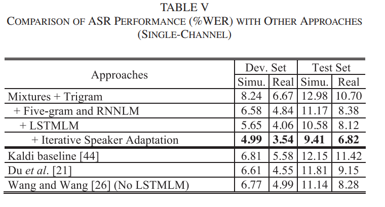


리뷰어의 제안으로 2번째 DNN 이후에 DNN 을 한번 더 하고 MVDR도 한번 더해서 WER 0.03%의 향상을 얻음
6. CONCLUSION
single-, multi- channel complex spectral mapping 으로 CHiME-4 에서 SOTA를 달성하였다.
TV-MVDR이 TI-MVDR 보다 더 좋은 ASR 결과를 보였다(특히 2 채널).
time-domain과 real-time, multi-speaker separation에 관해서 더 연구할 생각이다.
REFERENCE
[1] D. L. Wang and J. Chen, “Supervised speech separation based on deep learning: An overview,” IEEE/ACM Trans. Audio, Speech, Lang. Process., vol. 26, pp. 1702–1726, Oct. 2018.
[2] R. Haeb-Umbach et al., “Speech processing for digital home assistants: Combining signal processing with deep-learning techniques,” IEEE Signal Process. Mag., vol. 36, no. 6, pp. 111–124, Nov. 2019.
[3] S. Gannot, E. Vincent, S. Markovich-Golan, and A. Ozerov, “A consolidated perspective on multi-microphone speech enhancement and source separation,” IEEE/ACM Trans. Audio, Speech, Lang. Process., vol. 25, pp. 692–730, Apr. 2017.
[4] E. A. P. Habets and P. A. Naylor, “Dereverberation,” in Audio Source Separation and Speech Enhancement, E. Vincent, T. Virtanen, and S. Gannot, Eds. New York, NY, USA: Wiley, 2018, pp. 317–343.
[5] J. DiBiase, H. Silverman, and M. Brandstein, “Robust localization in reverberant rooms,” in Microphone Arrays, Berlin Heidelberg, Germany: Springer, 2001, pp. 157–180.
[6] T. Yoshioka et al., “The NTT CHiME-3 system: Advances in speech enhancement and recognition for mobile multi-microphone devices,” in Proc. IEEE Workshop Autom. Speech Recognit. Understanding, 2015, pp. 436–443.
[7] M. I. Mandel and J. P. Barker, “Multichannel spatial clustering for robust far-field automatic speech recognition in mismatched conditions,” in Proc. Interspeech, 2016, pp. 1991–1995.
[8] Z.-Q. Wang, X. Zhang, and D. L. Wang, “Robust speaker localization guided by deep learning based time-frequency masking,” IEEE/ACM Trans. Audio, Speech, Lang. Process., vol. 27, no. 1, pp. 178–188, Jan. 2019.
[9] J. Heymann, L. Drude, and A. Chinaev, and R. Haeb-Umbach, “BLSTM supported GEV beamformer front-end for the 3rd CHiME Challenge,” in Proc. IEEE Workshop Autom. Speech Recognit. Understanding, 2015, pp. 444–451.
[10] E. Vincent, S. Watanabe, A. A. Nugraha, J. Barker, and R. Marxer, “An analysis of environment, microphone and data simulation mismatches in robust speech recognition,” Comput. Speech Lang., vol. 46, pp. 535–557, 2017.
[11] T. Higuchi, N. Ito, T. Yoshioka, and T. Nakatani, “Robust MVDR beamforming using time-frequency masks for online/offline ASR in noise,” in Proc. IEEE Int. Conf. Acoustics, Speech Signal Process., 2016, pp. 5210–5214.
[12] H. Erdogan et al., “Improved MVDR beamforming using single-channel mask prediction networks,” in Proc. Interspeech, 2016, pp. 1981–1985.
[13] X. Zhang, Z.-Q. Wang, and D. L. Wang, “A speech enhancement algorithm by iterating single- and multi-microphone processing and its application to robust ASR,” in Proc. IEEE Int. Conf. Acoustics, Speech Signal Process., 2017, pp. 276–280.
[14] X. Xiao, S. Zhao, D. L. Jones, E. S. Chng, and H. Li, “On time-frequency mask estimation for MVDR beamforming with application in robust speech recognition,” in Proc. IEEE Int. Conf. Acoustics, Speech Signal Process., 2017, pp. 3246–3250.
[15] D. W. Griffin and J. S. Lim, “Signal estimation from modified short-time fourier transform,” IEEE Trans. Acoust., vol. 32, no. 2, pp. 236–243, Apr. 1984.
[16] T. Gerkmann, M. Krawczyk-Becker, and J. Le Roux, “Phase processing for single-channel speech enhancement: History and recent advances,” IEEE Signal Process. Mag., vol. 32, no. 2, pp. 55–66, Mar. 2015.
[17] Z.-Q. Wang, K. Tan, and D. L. Wang, “Deep learning based phase reconstruction for speaker separation: A trigonometric perspective,” in Proc.
IEEE Int. Conf. Acoustics, Speech Signal Process., 2019, pp. 71–75. [18] D. Williamson, Y. Wang, and D. L. Wang, “Complex ratio masking for monaural speech separation,” in Proc. IEEE/ACM Trans. Audio, Speech, Lang. Process., 2016, pp. 483–492.
[19] S.-W. Fu, T.-Y. Hu, Y. Tsao, and X. Lu, “Complex spectrogram enhancement by convolutional neural network with multi-metrics learning,” in Proc. IEEE Int. Workshop Mach. Learn. Signal Process., 2017, pp. 1–6.
[20] K. Tan and D. L. Wang, “Learning complex spectral mapping with gated convolutional recurrent networks for monaural speech enhancement,” in Proc. IEEE/ACM Trans. Audio, Speech, Lang. Process., 2020, pp. 380–390.
[21] J. Du, Y. Tu, L. Sun, F. Ma, H. Wang, and J. Pan, “The USTC–iFlytek system for CHiME-4 Challenge,” in Proc. CHiME-4, 2016, pp. 36–38.
[22] Y.-H. Tu et al., “An iterative mask estimation approach to deep learning based multi-channel speech recognition,” Speech Commun., vol. 106, pp. 31–43, 2019.
[23] Z.-Q. Wang and D. L. Wang, “Unsupervised speaker adaptation of batch normalized acoustic models for robust ASR,” in Proc. IEEE Int. Conf. Acoustics, Speech Signal Process., 2017, pp. 4890–4894.
[24] Z.-Q. Wang and D. L. Wang, “Mask-weighted STFT ratios for relative transfer function estimation and its application to robust ASR,” in Proc. IEEE Int. Conf. Acoustics, Speech Signal Process., 2018, pp. 5619–5623.
[25] Z.-Q. Wang and D. L. Wang, “On spatial features for supervised speech separation and its application to beamforming and robust ASR,” in Proc. IEEE Int. Conf. Acoustics, Speech Signal Process., 2018, pp. 5709–5713.
[26] P. Wang and D. L. Wang, “Utterance-wise recurrent dropout and iterative speaker adaptation for robust monaural speech recognition,” in Proc. IEEE Int. Conf. Acoustics, Speech Signal Process., 2018, pp. 4814–4818.
[27] S. Wisdom et al., “Differentiable consistency constraints for improved deep speech enhancement,” in Proc. IEEE Int. Conf. Acoustics, Speech and Signal Process., 2019, vol. 2019, pp. 900–904.
[28] Y. Jiang, D. L. Wang, R. Liu, and Z. Feng, “Binaural classification for reverberant speech segregation using deep neural networks,” IEEE/ACM Trans. Audio, Speech, Lang. Process., vol. 22, no. 12, pp. 2112–2121, Dec. 2014.
[29] S. Araki, T. Hayashi, M. Delcroix, M. Fujimoto, K. Takeda, and T. Nakatani, “Exploring multi-channel features for denoisingautoencoder-based speech enhancement,” in Proc. IEEE Int. Conf. Acoustics, Speech Signal Process., 2015, pp. 116–120. Authorized licensed use limited to: Sogang University Loyola Library. Downloaded on January 04,2021 at 03:29:07 UTC from IEEE Xplore. Restrictions apply. WANG et al.: COMPLEX SPECTRAL MAPPING FOR SINGLE- AND MULTI-CHANNEL SPEECH ENHANCEMENT AND ROBUST ASR 1787
[30] P. Pertilä and J. Nikunen, “Distant speech separation using predicted time-frequency masks from spatial features,” Speech Commun., vol. 68, pp. 97–106, 2015.
[31] X. Zhang and D. L.Wang, “Deep learning based binaural speech separation in reverberant environments,” IEEE/ACM Trans. Audio, Speech, Lang. Process., vol. 25, no. 5, pp. 1075–1084, May 2017.
[32] Z.-Q. Wang and D. L. Wang, “Combining spectral and spatial features for deep learning based blind speaker separation,” IEEE/ACM Trans. Audio, Speech, Lang. Process., vol. 27, no. 2, pp. 457–468, Feb. 2019.
[33] T. Yoshioka, H. Erdogan, Z. Chen, and F. Alleva, “Multi-microphone neural speech separation for far-field multi-talker speech recognition,” in Proc. IEEE Int. Conf. Acoustics, Speech Signal Process., 2018, pp. 5739–5743.
[34] Z.-Q.Wang, J. Le Roux, and J. R. Hershey, “Multi-channel deep clustering: discriminative spectral and spatial embeddings for speaker-independent speech separation,” in Proc. IEEE Int. Conf. Acoustics, Speech Signal Process., 2018, pp. 1–5.
[35] Y. Kubo, T. Nakatani, M. Delcroix, K. Kinoshita, and S. Araki, “Maskbased MVDR beamformer for noisy multisource environments: Introduction of time-varying spatial covariance model,” in Proc. IEEE Int. Conf. Acoustics, Speech Signal Process., 2019, pp. 6855–6859.
[36] S. Bai, J. Z. Kolter, and V. Koltun, “An empirical evaluation of generic convolutional and recurrent networks for sequence modeling,” 2018, arXiv:1803.01271.
[37] O. Ronneberger, P. Fischer, and T. Brox, “U-net: Convolutional networks for biomedical image segmentation,” inProc. MICCAI, 2015, pp. 234–241.
[38] G. Huang, Z. Liu, L. V. D. Maaten, and K. Q. Weinberger, “Densely connected convolutional networks,” in Proc. IEEE Conf. Comput. Vision Pattern Recognit., 2017, pp. 4700–4708.
[39] N. Takahashi, N. Goswami, and Y. Mitsufuji, “MMDenseLSTM: An efficient combination of convolutional and recurrent neural networks for audio source separation,” in Proc. 16th Int. Workshop Acoust. Signal Enhancement, Proc., 2018, pp. 106–110.
[40] Y. Liu and D. L. Wang, “Divide and conquer: A deep CASA approach to talker-independent monaural speaker separation,” in Proc. IEEE/ACM Trans. Audio, Speech, Lang. Process., 2019, pp. 2092–2102.
[41] J. Le Roux, S. Wisdom, H. Erdogan, and J. R. Hershey, “SDR – half-baked or well done?” in Proc. IEEE Int. Conf. Acoustics, Speech Signal Process., 2019, pp. 626–630.
[42] H. Erdogan, J. R. Hershey, S. Watanabe, and J. Le Roux, “Phase-sensitive and recognition-boosted speech separation using deep recurrent neural networks,” in Proc. IEEE Int. Conf. Acoustics, Speech Signal Process., 2015, pp. 708–712.
[43] J. Heymann and R. Haeb-Umbach, “Wide residual BLSTM network with discriminative speaker adaptation for robust speech recognition,” in Proc. CHiME-4, 2016, pp. 12–17.
[44] S.-J. Chen, A. S. Subramanian, H. Xu, and S. Watanabe, “Building state-of-the-art distant speech recognition using the CHiME-4 challenge with a setup of speech enhancement baseline,” in Proc. Interspeech, 2018, pp. 1571–1575.
[45] D. Yu and L. Deng, Automatic Speech Recognition: A Deep Learning Approach. Vienna, Austria, Springer, 2014.
[46] S. Bu, Y. Zhao, M.-Y. Hwang, and S. Sun, “A robust nonlinear microphone array postfilter for noise reduction,” in Proc. IWAENC, 2018, pp. 206–210.
[47] Y.-H. Tu, J. Du, N. Zhou, and C.-H. Lee, “Online LSTM-based iterative mask estimation for multi-channel speech enhancement and ASR,” inProc. Annu. Summit Conf. Signal Inf. Process., 2018, pp. 362–366.
[48] K. Shimada, Y. Bando, M. Mimura, K. Itoyama, K. Yoshii, and T. Kawahara, “Unsupervised speech enhancement based on multichannel NMF-informed beamforming for noise-robust automatic speech recognition,” IEEE/ACM Trans. Audio, Speech, Lang. Process., vol. 27, no. 5, pp. 960–971, May 2019.


